This post covers the concept of zero-shot image classification with an example. It is the process where a model can classify images without being trained on a particular use case.
Fundamentals
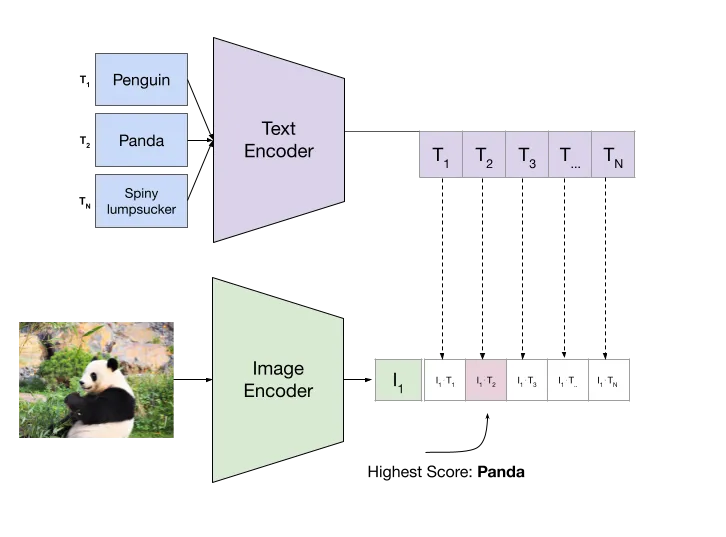
To make this work, we need a Multimodal embedding model and a vector database. Let's start with something called CLIP, which stands for Contrastive Language-Image Pre-Training.
CLIP acts like a versatile interpreter for various types of data, including images, text, and more. It achieves this through two key components: a Text Encoder and an Image Encoder, both trained to understand these inputs within the same vector space. During training on 400 million internet-collected image-text pairs, CLIP learned to place similar pairs close together in this space while separating dissimilar pairs.
Key features of CLIP include:
- It operates without the need for datasets labeled with specific class categories, relying instead on image-text pairs where the text describes the image.
- Rather than extracting features from images using traditional CNNs, CLIP leverages more detailed text descriptions, enhancing its feature extraction capabilities.
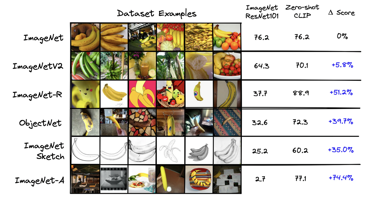
- In performance tests, CLIP demonstrated superior zero-shot classification compared to a fine-tuned ResNet-101 model on datasets derived from ImageNet, showcasing its robust understanding of diverse datasets beyond its specific training data.
How does CLIP work
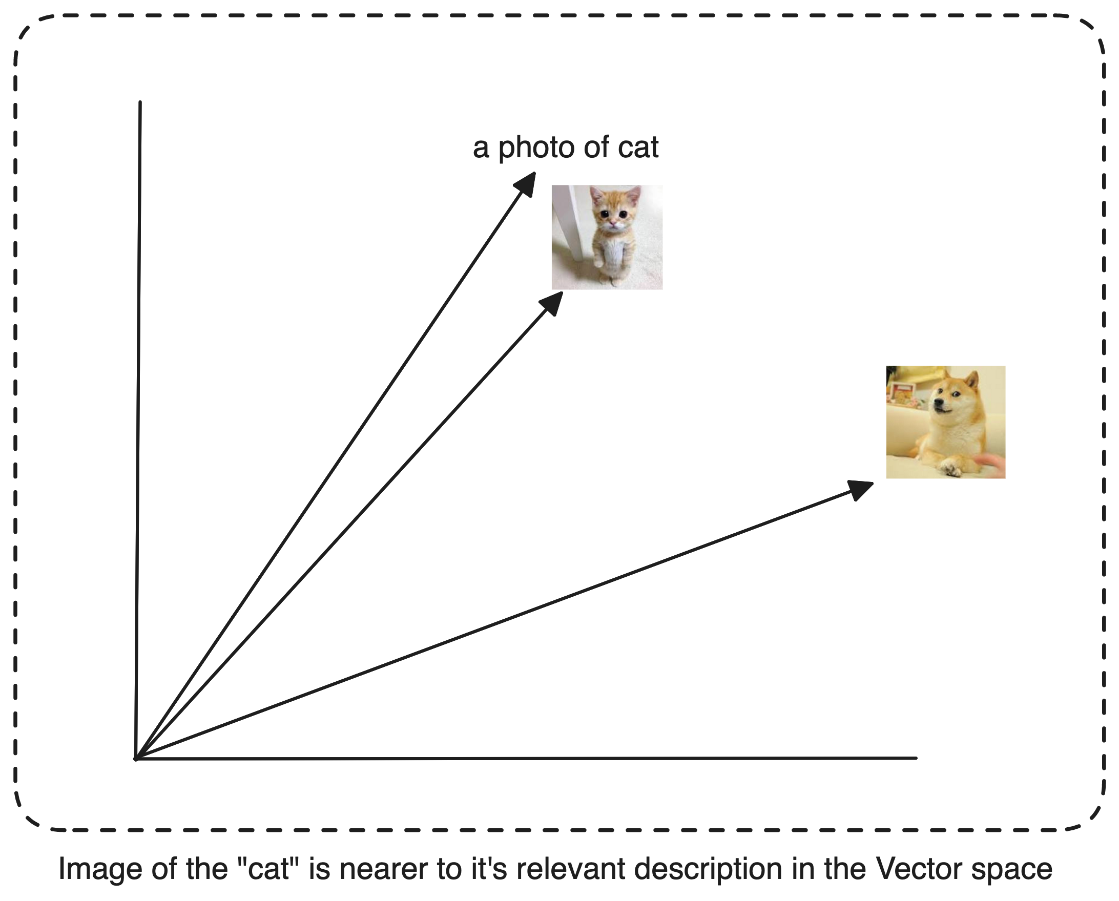
In traditional CNN-based classification, images are labeled with specific classes, and the model learns to recognize features that distinguish between these classes through supervised training. In contrast, zero-shot classification utilizes a Text Encoder and an Image Encoder that produce 512-dimensional vectors for both images and text. These vectors are mapped to the same semantic space, meaning an image vector for "cat" is similar to the vector of a text description like "a photo of a cat".
By leveraging this shared vector space, zero-shot classification allows the model to classify images into categories it hasn't seen during training. Instead of relying solely on predefined class labels, the model compares the vector representation of a new image to vectors representing textual descriptions of various categories, enabling it to generalize across unseen classes.
To optimize our zero-shot classification, it's beneficial to transform class labels from basic words like "cat," "dog," and "horse" into descriptive phrases such as "a photo of a cat," "a photo of a dog," or "a photo of a horse." This transformation mirrors the text-image pairs used during the model's pretraining, where prompts like "a photo of a {label}" were paired with each label to create training examples [1]. You can play around with the prompts and see how CLIP performs.
Vector Index
To power our zero-shot classification system, we'll use a vector database to store labels and their embeddings.
Implementation
You can also follow along with this colab


Let's take a look at an example. For this demonstration, I'll use the uoft-cs/cifar100 dataset from Hugging Face Datasets.
from datasets import load_dataset

imagedata = load_dataset(
    'uoft-cs/cifar100',
    split="test"
)

imagedata
Let’s see original label names
# labels names
labels = imagedata.info.features['fine_label'].names
print(len(labels))
labels
100

['apple',
 'aquarium_fish',
 'baby',
 'bear',
 'beaver',
 'bed',
 'bee',
 'beetle',
 'bicycle',
 'bottle',
 'bowl',
 'boy',
 'bridge',
 'bus',
 'butterfly',
 'camel',
 'can',
 'castle',
 'caterpillar',
 'cattle',
 'chair',
 'chimpanzee',
 'clock',
 'cloud',
 'cockroach',
...
 'whale',
 'willow_tree',
 'wolf',
 'woman',
 'worm']
Looks good! We have 100 classes to classify images from, which would require a lot of computing power if you go for traditional CNN. However, let's proceed with our zero-shot image classification approach.
Let’s generate the relevant textual descriptions for our labels. (This step is optional recommendation covered in previous section.)
# generate sentences
clip_labels = [f"a photo of a {label}" for label in labels]
clip_labels
Now let’s initialize our CLIP embedding model, I will use the CLIP implementation from Hugging face.
import torch
from transformers import CLIPProcessor, CLIPModel

model_id = "openai/clip-vit-large-patch14"
processor = CLIPProcessor.from_pretrained(model_id)
model = CLIPModel.from_pretrained(model_id)

device = "cuda" if torch.cuda.is_available() else "cpu"
model.to(device)
We'll convert our text descriptions into integer representations called input IDs, where each number stands for a word or subword, more formally tokens. We'll also need an attention mask to help the transformer focus on relevant parts of the input.
label_tokens = processor(
    text=clip_labels,
    padding=True,
    return_tensors='pt'
).to(device)

# Print the label tokens with the corresponding text
for i in range(5):
    token_ids = label_tokens['input_ids'][i]
    print(f"Token ID : {token_ids}, Text : {processor.decode(token_ids, skip_special_tokens=False)}")
Token ID : tensor([49406,   320,  1125,   539,   320,  3055, 49407, 49407, 49407]), Text : <|startoftext|>a photo of a apple <|endoftext|><|endoftext|><|endoftext|>
Token ID : tensor([49406,   320,  1125,   539,   320, 16814,   318,  2759, 49407]), Text : <|startoftext|>a photo of a aquarium _ fish <|endoftext|>
Token ID : tensor([49406,   320,  1125,   539,   320,  1794, 49407, 49407, 49407]), Text : <|startoftext|>a photo of a baby <|endoftext|><|endoftext|><|endoftext|>
Token ID : tensor([49406,   320,  1125,   539,   320,  4298, 49407, 49407, 49407]), Text : <|startoftext|>a photo of a bear <|endoftext|><|endoftext|><|endoftext|>
Token ID : tensor([49406,   320,  1125,   539,   320, 22874, 49407, 49407, 49407]), Text : <|startoftext|>a photo of a beaver <|endoftext|><|endoftext|><|endoftext|>
Now let’s get the CLIP embeddings
# encode tokens to sentence embeddings from CLIP

with torch.no_grad():
    label_emb = model.get_text_features(**label_tokens) # passing the label text as in "a photo of a cat" to get it's relevant embedding from clip model

# Move embeddings to CPU and convert to numpy array
label_emb = label_emb.detach().cpu().numpy()
label_emb.shape
(100, 768)We now have a 768-dimensional vector for each of our 100 text class sentences. However, to improve our results when calculating similarities, we need to normalize these embeddings.
Normalization helps ensure that all vectors are on the same scale, preventing longer vectors from dominating the similarity calculations simply due to their magnitude. We achieve this by dividing each vector by the square root of the sum of the squares of its elements. This process, known as L2 normalization, adjusts the length of our vectors while preserving their directional information, making our similarity comparisons more accurate and reliable.
import numpy as np
# normalization
label_emb = label_emb / np.linalg.norm(label_emb, axis=0)
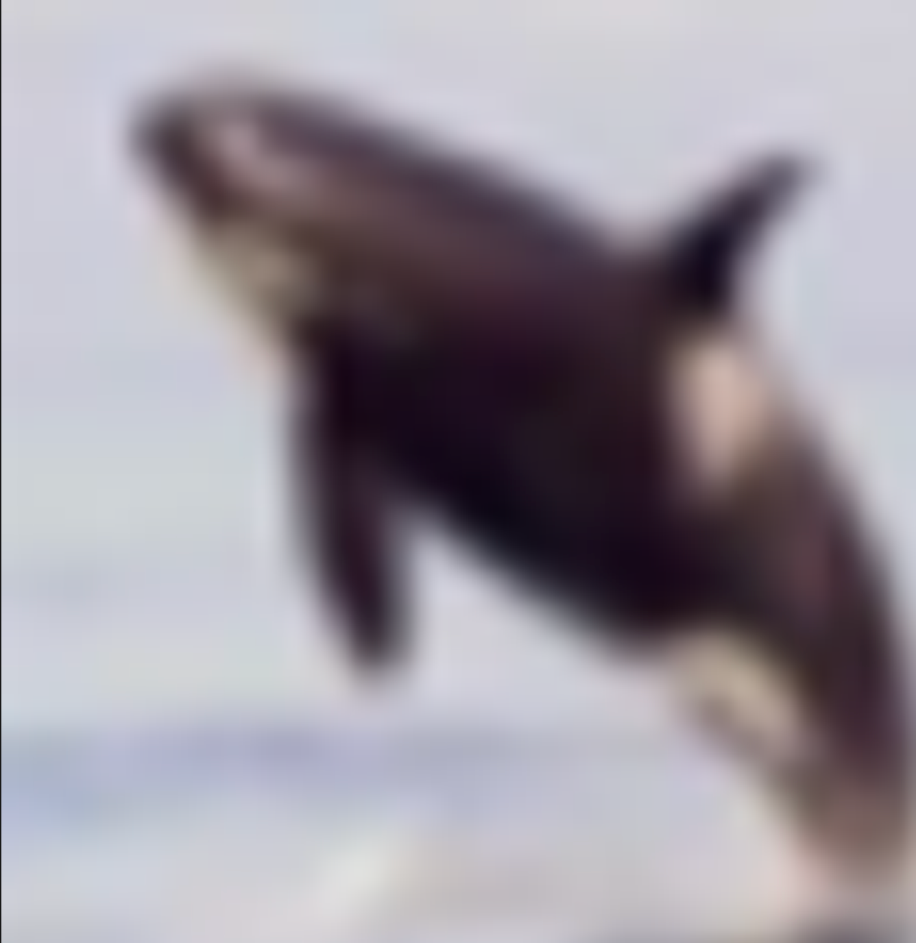
label_emb.min(), label_emb.max()Ok, let’s see a random image from our dataset
import random

index = random.randint(0, len(imagedata)-1)
selected_image = imagedata[index]['img']
selected_image
First, we'll run the image through our CLIP processor. This step ensures the image is resized first, then the pixels are normalized, then converting it into the tensor and finally adding a batch dimension.
image = processor(
    text=None,
    images=imagedata[index]['img'],
    return_tensors='pt'
)['pixel_values'].to(device)
image.shape
torch.Size([1, 3, 224, 224])
Now here this shape represents a 4-dimensional tensor:
- 1: Batch size (1 image in this case)
- 3: Number of color channels (Red, Green, Blue)
- 224: Height of the image in pixels
- 224: Width of the image in pixels
So, we have one image, with 3 color channels, and dimensions of 224x224 pixels. Now we'll use CLIP to generate an embedding.
img_emb = model.get_image_features(image)
img_emb.shape
torch.Size([1, 768])
We'll use LanceDB to store our labels, with their corresponding embeddings to allow performing vector search across the dataset.
import lancedb
import numpy as np

data = []
for label_name, embedding in zip(labels, label_emb):
    data.append({"label": label_name, "vector": embedding})

db = lancedb.connect("./.lancedb")
table = db.create_table("zero_shot_table", data, mode="Overwrite")

# Prepare the query embedding
query_embedding = img_emb.squeeze().detach().cpu().numpy()
# Perform the search
results = (table.search(query_embedding)
           .limit(10)
           .to_pandas())

print(results.head(n=10))
|   label         | vector | distance |
|-----------------|-----------------------------------------------------------|-------------|
| whale           | [0.05180167, 0.008572296, -0.00027403078, -0.12351207, ...]| 447.551605  |
| dolphin         | [0.09493398, 0.02598409, 0.0057568997, -0.13548125, ...]| 451.570709  |
| aquarium_fish   | [-0.094619915, 0.13643932, 0.030785343, 0.12217164, ...]| 451.694672  |
| skunk           | [0.1975818, -0.04034014, 0.023241673, 0.03933424, ...]| 452.987640  |
| crab            | [0.05123004, 0.0696855, 0.016390173, -0.02554354, ...]| 454.392456  |
| chimpanzee      | [0.04187969, 0.0196794, -0.038968336, 0.10017315, ...]| 454.870697  |
| ray             | [0.10485967, 0.023477506, 0.06709562, -0.08323726, ...]| 454.880524  |
| sea             | [-0.08117988, 0.059666794, 0.09419422, -0.18542227, ...]| 454.975311  |
| shark           | [-0.01027703, -0.06132377, 0.060097754, -0.2388756, ...]| 455.291901  |
| keyboard        | [-0.18453166, 0.05200073, 0.07468183, -0.08227961, ...]| 455.424866  |
Here are the results. Our initial accurate prediction is a whale, demonstrating the closest resemblance between the label and the image with minimal distance, just as we had hoped. What's truly remarkable is that we achieved this without running a single epoch for a CNN model. That’s zero shot classification for you fellas. Here is the colab for your reference. See you in next one.
Checkout more examples on VectorDB-recipes