I came upon a blog post yesterday benchmarking LanceDB. The numbers looked very surprising to me, so I decided to do a quick investigation on my own. First, I want to express gratitude to the post’s author for taking the time to do a run down and publishing their results. Running these benchmarks is often a tedious exercise in chasing down details and analyzing tradeoffs. If we feel something was missed in a benchmark of LanceDB, I believe it’s the fault of our documentation and not the fault of the author.

TL;DR: LanceDB is fast, and achieves <20ms latencies (going as low as 1 ms) across all configurations in the GIST-1M benchmark dataset.

Benchmark setup

We use the same GIST-1M dataset referred to in the original benchmark. This can be found at the source: http://corpus-texmex.irisa.fr/ (gist.tar.gz).

The benchmarks shown in this post were performed on a 2022 Macbook Pro (M2 Max). When using LanceDB, hardware can make a difference. Because LanceDB is primarily disk-based for both indexing and storage, it benefits greatly from a fast disk — it’s highly recommended to use an SSD instead of older HDDs. While most other vector DBs that use in-memory indexes are sensitive to the amount of RAM, LanceDB is much less memory-intensive.

The original blog post used v0.3.1of LanceDB. Because the system is continually improving, I ran these benchmarks using the latest LanceDB v0.3.6 (and latest lance python v0.8.21).

You can find the code to reproduce the benchmarks here.

• Download gist.tar.gzfrom the source and unzip
• Generate Lance datasets using the datagen.py script:
• Database vectors:

./datagen.py ./gist/gist_base.fvecs ./.lancedb/gist1m.lance -g 1024 -m 50000 -d 960

• Query vectors:

./datagen.py ./gist/gist_query.fvecs ./.lancedb/gist_query.lance -g 1024 -m 50000 -d 960 -n 1000

• Create index with 256 partitions and 120 subvectors:

./index.py ./.lancedb/gist1m.lance -i 256 -p 120

• Run the benchmark for recall@1:

./metrics.py ./.lancedb/gist1m.lance results.csv -i 256 -p 120 -q ./.lancedb/gist_query.lance -k 1

The benchmark results will be output to results.csv .

Indexing

The original post set the num_partitionsas 256 or 512, and num_sub_vectorsas either 120 or 240. Across all combinations, the blog post reported >1000 sec indexing times using a T4 GPU, which was surprising. In addition, at this scale, a GPU really isn’t necessary for indexing. On my macbook, I timed the indexing job using just my CPU, for a total wall time on the order of 1 minute:

Even without a GPU, the indexing times should be fast enough on a dataset of size 1M.

Querying

The original post varied nprobes during querying. The author calculated recall@1 for 20 or 40 nprobes, reporting 0.65 to 0.9 recall at 45 to 177ms latencies. For LanceDB, a key parameter that can make an impact is the refine_factor. By setting this parameter, the user can tell LanceDB to compute the full vector distance (instead of just the PQ distance) for a small subset of the results to get a much better recall for a small latency penalty of less than a millisecond on datasets of this size.

Refine Factor

LanceDB uses PQ, or Product Quantization, to compress vectors and speed up search. However, because PQ is a lossy compression algorithm, it can significantly reduce recall. To combat this problem, we introduce a process called refinement. The normal process computes distances using the compressed PQ vectors. We then take the most similar PQ vectors, and refine the results by fetching the actual vectors and computing the full vector distance and reordering based on those scores.

If you are retrieving the top 10 results and set refine_factorto 5, then LanceDB will fetch the 50 most similar vectors (according to PQ), compute the distances again based on full vectors for those 50, then rerank based on those scores.

Results

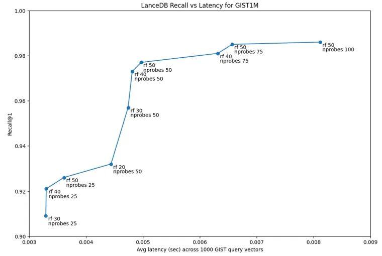
Using the ivf256 and pq120 index I created in my version of the benchmark, I tested recall@1 using the 1000 query vector set provided by GIST across an nprobesand a refine_factor frontier. As you can see, 3ms latency is sufficient to get above 0.9 recall (nprobes 25 and rf 30). And 5ms is sufficient for 0.95 recall (nprobes 50 and rf 30):

The full table of results that generated this graph is published on github.

3ms latency is sufficient to get above 0.9 recall (nprobes 25 and rf 30). And 5ms is sufficient for 0.95 recall (nprobes 50 and rf 30)

We can zoom in a little bit and focus on the high recall range above 0.9 recall, there’s a fairly wide variety of refine / nprobes that delivers this recall in single digit milliseconds, which means we don’t have to be too sensitive to finding exactly the right configurations here.

Linux

Given that the original benchmark’s author was using a T4 GPU, I’m guessing it was done on a Linux machine. So I also ran the same benchmark on Linux (Lenovo P52 with Xeon E-2176M 12-core CPU). This laptop is roughly 5 years old, so we’d expect the indexing performance to not be as good as a modern Macbook. However, we show below that it’s still almost an order of magnitude faster than what was reported in the original blog post.

It’s clear that the wall time duration for indexing is 2min 46sec.

As expected, the query benchmarks for the older CPU on Linux are slightly slower than on the Macbook, but still very low, ranging from roughly 7–20ms for recall@1 above 0.9.

You can achieve even more performance if you’re using Linux. Currently, our PyPI build is not as optimized as it could be in order to be compatible with some of the older AWS Lambda CPUs (Haswell). If you’re on a newer generation CPU like Skylake / Icelake, you can get much better performance by building the underlying Lance artifact from source using RUSTFLAGS=’-C target-cpu=native’ maturin develop -r . In the future we’ll be tackling this so the workaround is not necessary. This is tracked here: https://github.com/lancedb/lance/issues/1733.

A Different Architecture

The author rightly noted that LanceDB is different because it’s an embedded database that can run inside your application without having to deal with additional infrastructure. This is certainly one reason why a lot of users have chosen LanceDB.

There’s another big reason that makes LanceDB different. Because the index is disk-based, it means that LanceDB’s memory requirements are very low. A lot of our users actually store data on S3 and use LanceDB to query their S3 object files directly from AWS Lambda or their own application. And with the recent announcement of S3 Express, LanceDB will be able to deliver even more performance.

Many of our users actually store data on S3 and use LanceDB to query their S3 object files directly from AWS Lambda

LanceDB is also among the very few serverless vector databases that actually allows you to separate compute from storage. In OLTP databases, Neon is a great example of the same type of architecture. Nikita Shamgunov, the founder of Neon, posted a great thread explaining the implications of this:

For LanceDB, the implication is that scaling up means getting a bigger disk (or network drive), which is a lot simpler and far less expensive than sharding data across a lot of nodes or buying terabytes of RAM.

Also, LanceDB is fast. I’m able to search through 1 billion vectors (128D) on my macbook in <100ms:

Searching over 1B vectors on a single node in under 100 ms

Conclusion

In this blog, we’ve seen how appropriately setting the refine_factor boosted the recall@1 to 0.95 while still delivering a latency of about 5ms. The indexing time is also quite fast at around 60s for 1M 960D vectors. The key lesson learned for us is that having great technology isn’t enough — we also need to make our documentation much better so users aren’t missing such an important parameter to tune their searches if they need high recall.

In the coming weeks, we’ll also be publishing benchmarks with code that you can run and replicate on your own datasets, so you can more confidently decide on what tool to proceed with for your RAG and other vector search applications. Stay tuned!