Columnar File Readers in Depth: Column Shredding

Record shredding is a classic method used to transpose rows of potentially nested data into a flattened tree of buffers that can be written to the file. A similar technique, cascaded encoding, has recently emerged, that converts those arrays into a flattened tree of compressed buffers. In this article we explain and connect these ideas, but also explore the impacts of all this shredding on our goal of random access I/O, which leads to new approaches such as reverse shredding.

Record Shredding Overview

At the start of our journey we typically have some kind of row-based table, or perhaps it is a stream of events, or maybe a vector of objects. All of these are "row based" structures and they are extremely intuitive to work with and a natural representation of data. This is typically the format that data arrives at our database and the format that data emerges from our database.

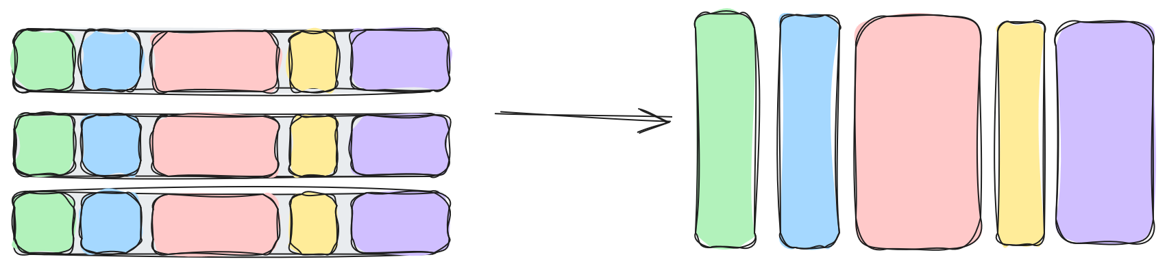
Unfortunately, this format is not great for bulk processing or storage. There are a lot of specific reasons for this but the general idea is that we don't typically operate on all of our columns at once. Working with data we don't need has costs (I/O, cache, etc.) As a result, we need to transpose our data from a row-based structure to a column-based structure.

Level 1: Table -> Columns

The first level of transpose is the simplest one. We split the table into columns. If we're lucky to have simplistic data, like a 2D matrix, or a spreadsheet, then this basically completes our journey. However, realistic data is rarely so simple. In fact, you might not even think you have a table. Tables are 2D structures after all and our objects don't feel quite so flat and two dimensional.

My first deep dive into data analysis (an indeterminate number of years ago) dealt with results from a manufacturing test system. Each time a test ran it would generate a test result. The test result had some basic properties (date of test, id & version of device under test, id & version of test equipment, etc.) but also some nested properties. For example, there were various tests that would run and each would run 20 iterations at different test frequencies and we would measure a score for each input frequency.

For now, let's pretend our test results are in YAML and we receive one row per YAML test result and that looks something like this:

timestamp: 514883700000
dut_sn: "D0N70P3ND34D1N51D3"
dut_version: "123.45"
bench_sn: "5H4K35H4K35H4K35H4K3"
tests:
  rise_time:
    - frequency: 10
      value: 0.3
    - frequency: 20
      value: 0.5
    - frequency: 30
      value: 0.2
    - frequency: 40
      value: 0.45
  settling_time:
    - frequency: 10
      value: 0.4
    - frequency: 20
      value: 0.6
    - frequency: 30
      value: 0.3
    - frequency: 40
      value: 0.55

If we only apply a single level of transpose we get five columns, "timestamp", "dut_sn", "dut_version", "bench_sn", and "tests". This last column (tests) is tricky. There are multiple columns inside of it and even a nested list of values. One classic strategy to deal with this problem (or, more accurately, not deal with it) is to just convert the "tests" column into a JSON object.

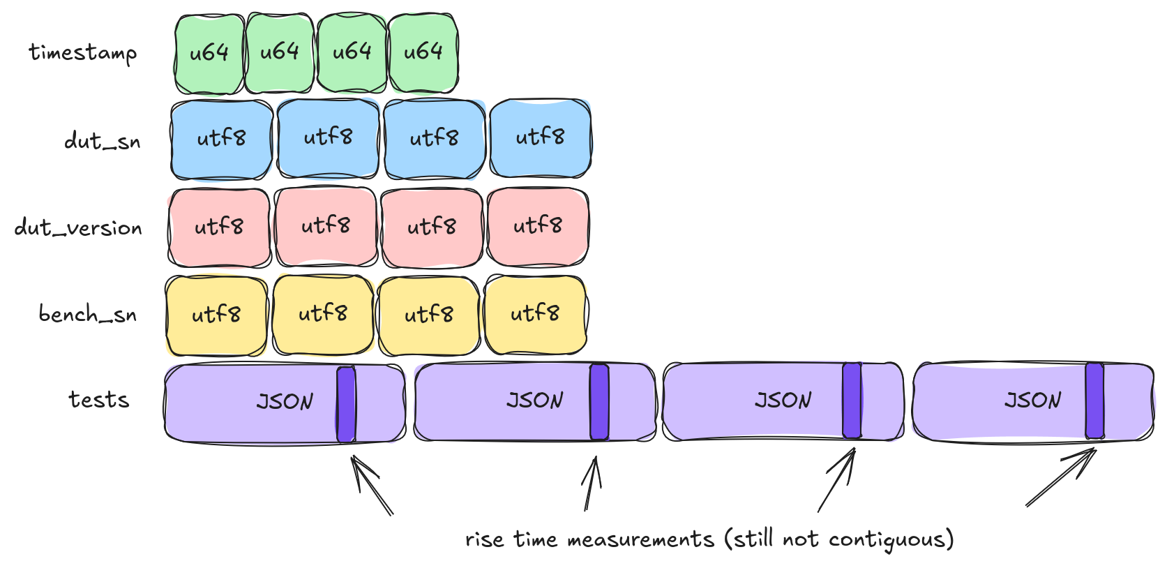
There are several issues with this strategy, but today we're focused on I/O. So let's ignore the JSON encode / decode cost. The main problem is that it still mixes unrelated data into our data of interest. For example, if we want to analyze our rise_time experiments we still are going to suffer because those values are bunched together with settling_time. Fortunately, we can do better.

Level 2: Column -> Array

Our first pass gave a rather simple transposition of our data. We are now working with columns and not rows. However, some of these columns are nested columns, and those are basically little rows. We can do better. We can shred.

At this next level we are going to convert a sequence of columns into a flattened sequence of arrays. To do this we need to look in more detail at the struct array.

Structs

For clarity, by "struct" I am talking about a high level concept, and not any specific language feature. In JSON & YAML we'd call these "objects". In XML we'd call them elements. In Arrow we call them structs. Looking at our above test result example we have tests which is a struct. It has two child fields rise_time and settling_time. To shred this, all we need to do is split out each child array.

However...there is one small sticking point (isn't there always), which is nullability. Consider the following YAML representation of three points (7, 3), NULL, (NULL, 5):

- point:
    x: 7
    y: 3
- point: null
- point:
    x: null
    y: 5

If we just split this into two different arrays we would get:

point.x:
 - 7
 - null
 - null
point.y:
 - 3
 - null
 - 5

But then, when we reassemble this, we could also get:

- point:
    x: 7
    y: 3
- point:
    x: null
    y: null
- point:
    x: null
    y: 5

Note that this isn't quite the same as what we started with. Interestingly, the solution to this problem is right about where Arrow, Parquet, and ORC start to diverge. That being said, none of these solutions operate at Level 2, and so there is no real reference solution at this layer. In the interest of fun, let's invent one real quick, sticking with our YAML.

point.x:
 - value: 7
 - nonvalue: 1 
 - nonvalue: 0
point.y:
 - value: 3
 - nonvalue: 1
 - value: 5

This is a level 2 YAML encoding of our points. We encode every item as an object with one of two properties. If the object has the value property it points to the value. If the object has the nonvalue property it points to a special integer. If this special integer is 0 then the item itself is null. If it is non-zero then you have to walk that far up the structure tree to find the actually null (e.g. 1 means "parent is null", 2 means "grandparent is null", etc.)

What about lists? At level 2, we are just moving from columns to arrays. A list is already a single array. There isn't anything we have to do here. All we are doing at level 2 is flattening out structs. We will see lists soon in level 3.

Level 3: Array -> Buffer

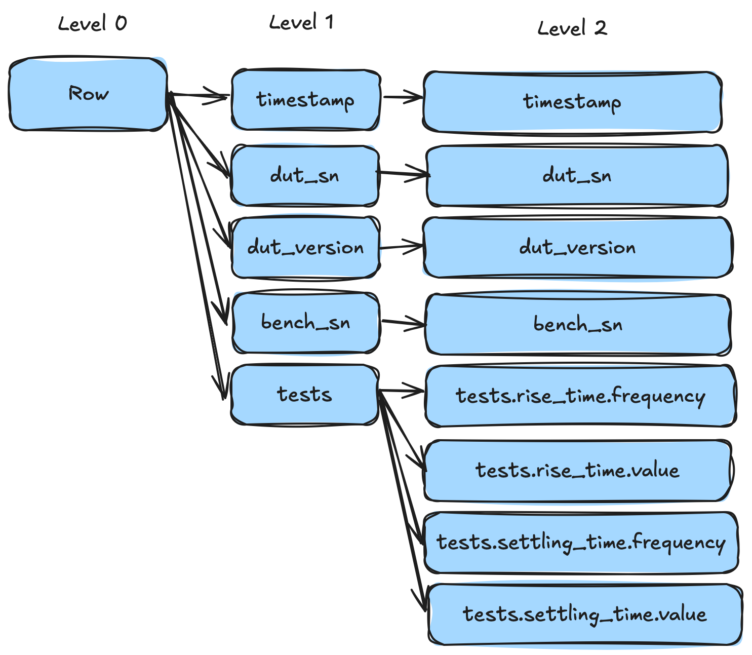
By this point, things are feeling pretty column-oriented. To get further, we have to really start thinking about "what is an array really?" As an example, let's look at our original manufacturing test example. Stopping after level 2 we have:

timestamp: 514883700000
dut_sn: "D0N70P3ND34D1N51D3"
dut_version: "123.45"
bench_sn: "5H4K35H4K35H4K35H4K3"
tests.rise_time.frequency:
  - - 10
    - 20
    - 30
    - 40
tests.rise_time.value:
  - - 0.3
    - 0.5
    - 0.2
    - 0.45
tests.settling_time.frequency:
  - - 10
    - 20
    - 30
    - 40
tests.settling_time.value:
  - - 0.4
    - 0.6
    - 0.3
    - 0.55

Let's pretend we took a few more measurements and let's zoom in on just the tests.rise_time.frequency column.

tests.rise_time.value:
  - - 0.3
    - 0.5
    - 0.2
    - 0.45
  - - 0.33
    - 0.43
    - 0.25
    - 0.4
  - - 0.5
    - 0.32
    - 0.6
    - 0.1

Again, it sure looks pretty columnar. But..."what is a list really?" Or, more concretely, what does this look like in RAM (and/or storage)? Let's take a look at the memory representation we get from the naive python representation of [[0.3, 0.5, 0.2, 0.45], [0.33, 0.43, 0.25, 0.4], [0.5, 0.32, 0.6, 0.1]]

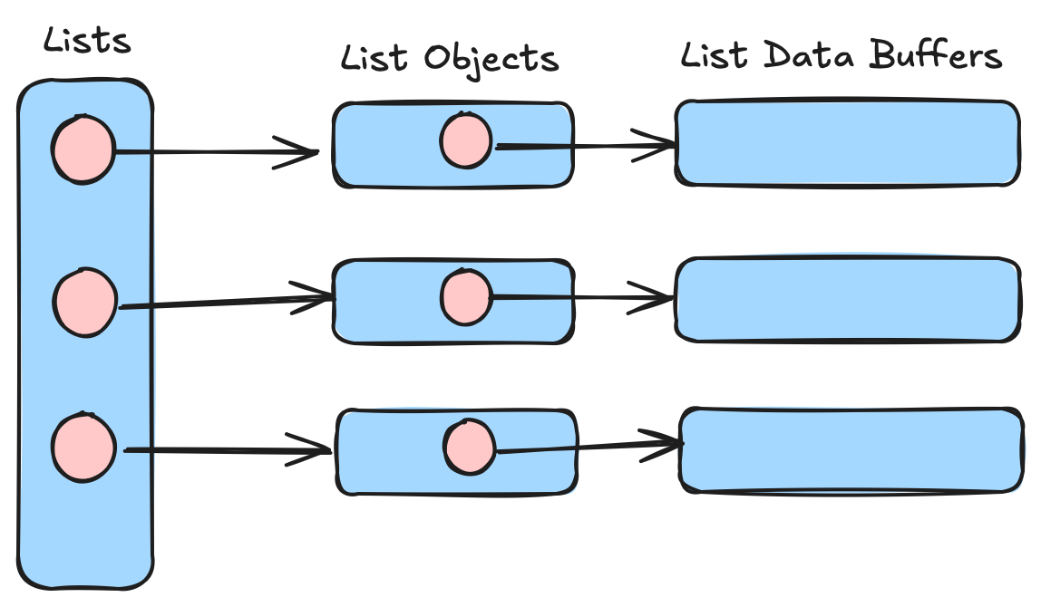
A "list of lists" in this case is a contiguous array of objects, each pointing to a list object (which contains data like the list size, etc.). Each list object then points to a contiguous array of values. Our data is scattered all over the place. This is "not great"™️ for columnar analytics. Now we can understand our goal for level 3. We want to go from a flattened sequence of arrays to a flattened sequence of buffers.

Decomposing lists

There is at least two ways we can turn a list array into a sequence of flattened buffers. In Arrow and ORC we use "offsets + values". In Parquet we use repetition levels. Repetition levels are more complicated, and I'm going to talk about them in a future post, so let's look at the "offsets + values" approach instead. Once again, we can visualize this using YAML.

tests.rise_time.value.offsets:
  - 0
  - 4
  - 8
  - 12
tests.rise_time.value.values:
  - 0.3
  - 0.5
  - 0.2
  - 0.45
  - 0.33
  - 0.43
  - 0.25
  - 0.4
  - 0.5
  - 0.32
  - 0.6
  - 0.1

The values buffer is a single contiguous buffer of flattened values. The offsets buffer is a single contiguous buffer of offsets. If we want to find the list at index i we just need to grab offsets[i] and offsets[i+1]. For more complete examples, including lists with varying numbers of items, you can look up Arrow tutorials (or even the reference itself).

Revisiting Structs

Now that we have this third level of shredding we can look at the Arrow approach to solving the struct nullability problem. In Arrow (and ORC), nullability (or more intuitively, "validity") is a separate bit buffer that stores a 1 for each non-null entry and a 0 for each null entry. Let's put all this together and look at our original manufacturing test data, but now split into buffers using Arrow's encoding scheme.

I keep mentioning that Parquet's encoding scheme is different, but it is still accomplishing the same goal. Without going into great detail let's look at the same data with Parquet's encoding scheme. This difference in schemes is rather interesting. Note that one of them feels more "transparent" 😉

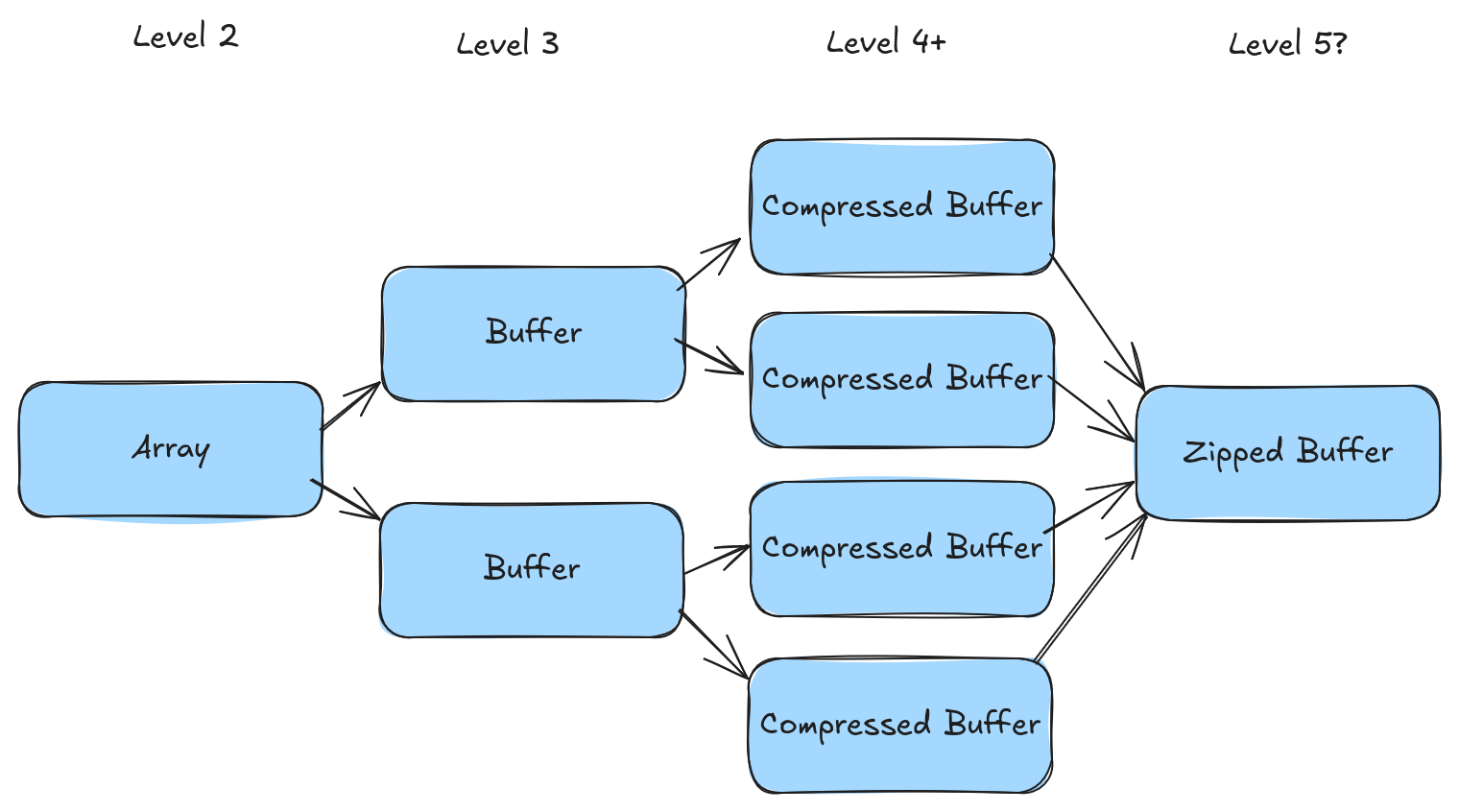
Level 4+: Buffer -> Compressed Buffer

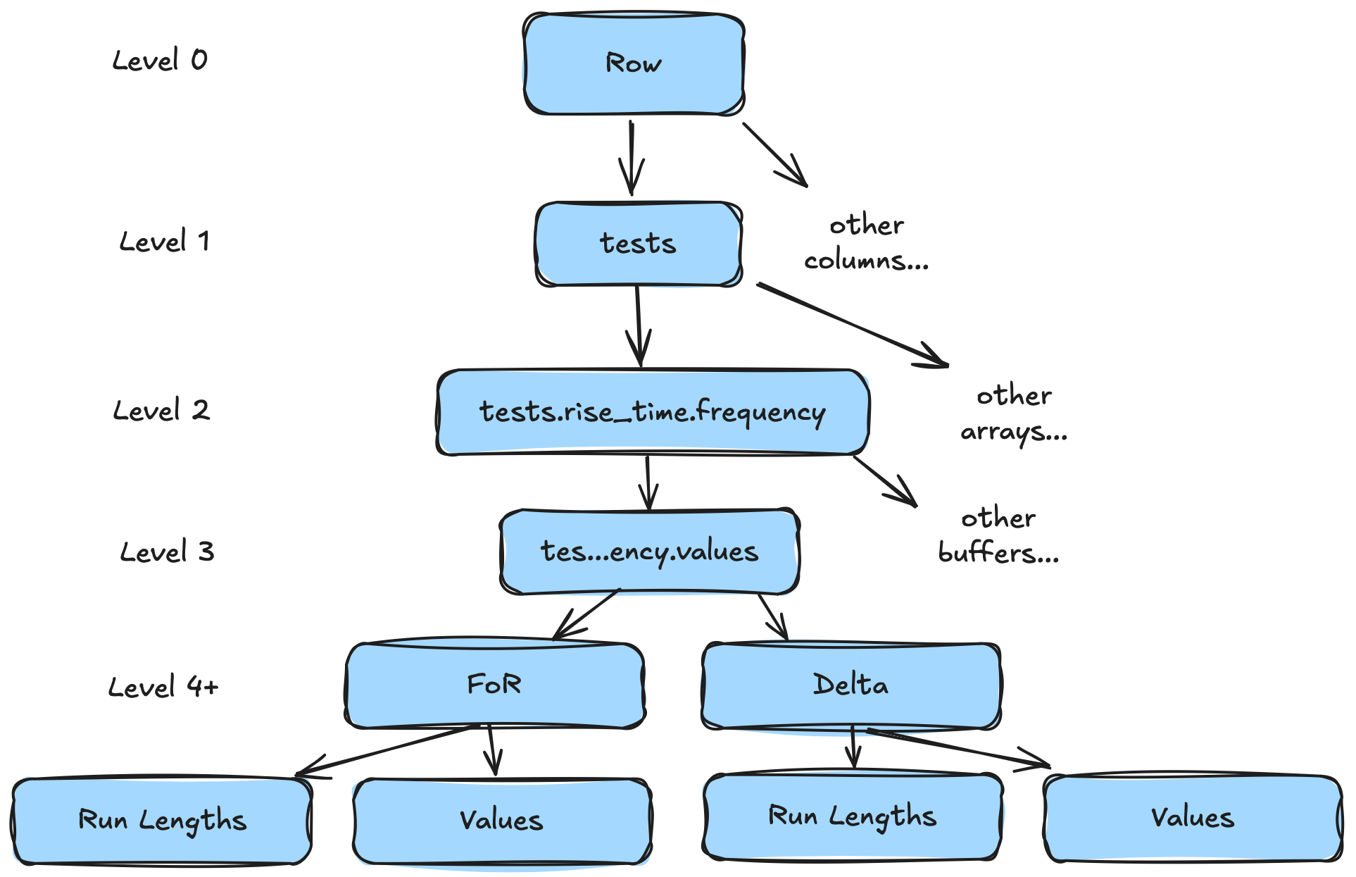
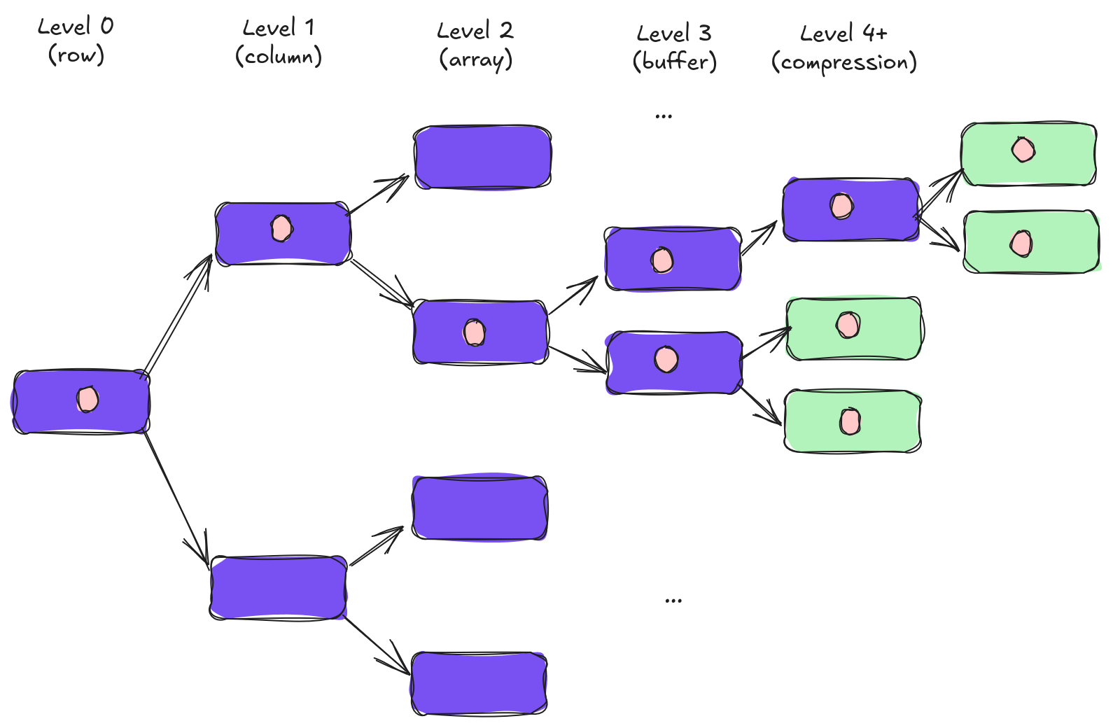
At this point our data has been shredded into nice contiguous buffers. Most tutorials on shredding will stop here. We won't. We...can...shred...more!

We've seen that we can look at our shredding so far as a tree of operations that brought us from our root node (a row) to a series of leaf nodes (the buffers). A relatively recent paper (BtrBlocks) pointed out that compression can also be viewed in this way. In fact, compression can, in some ways, be thought of as just more layers of shredding. We can split a single buffer into a flattened sequence of buffers, where the sum of our leaf buffers is smaller than the original buffer.

Let's look at an example. Again, let's pretend we have three rows but now we can look at the frequency value (a list of integers):

tests.rise_time.frequency.offsets:
 - 0
 - 4
 - 8
 - 12
tests.rise_time.frequency.values:
 - 10
 - 20
 - 30
 - 40
 - 10
 - 20
 - 30
 - 40
 - 10
 - 20
 - 30
 - 40

Both of these buffers look pretty compressible to me. There are a lot of patterns in the data (compression is the art of exploiting patterns). Let's cheat and use some a priori knowledge that we're repeating in groups of 4. We can apply a "frame-of-reference + delta" encoding in chunks of 4.

tests.rise_time.frequency.offsets:
 - 0
 - 4
 - 8
 - 12
tests.rise_time.values.chunk_width: 4
tests.rise_time.values.frame_of_reference:
 - 0
 - 0
 - 0
tests.rise_time.values.delta:
 - 10
 - 10
 - 10
 - 10
 - 10
 - 10
 - 10
 - 10
 - 10
 - 10
 - 10
 - 10

Now we've got even better patterns. Those are constant arrays. We can decompose those even further with "run length encoding".

tests.rise_time.frequency.offsets:
 - 0
 - 4
 - 8
 - 12
tests.rise_time.values.chunk_width: 4
tests.rise_time.values.frame_of_reference.values:
 - 0
tests.rise_time.values.frame_of_reference.run_lengths:
 - 3
tests.rise_time.values.delta.values:
 - 10
tests.rise_time.values.delta.run_lengths:
 - 12

So now we've shredded a single buffer (tests.rise_time.values) with 12 elements into four different buffers, each with a single element. In fact, we added two different levels to our tree. Each compression technique adding a new level.

Too Much Shredding?

Is there such a thing as too much shredding? No, of course not, this is the wonder of vectorized compute. We get great compression and great scan performance, what's not to like.

Yes, possibly, once we start to consider random access patterns. To understand why let's imagine we want to read a single value. In other words, one column value on one particular row (if you're thinking in spreadsheet terms this would be one cell). For example, maybe we want to grab the "vector column" in the 400th row because our secondary index tells us it's a potential match. Let's look what happens to that value as we shred our data.

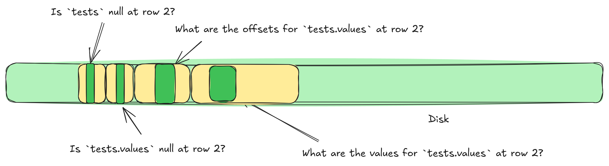
Initially, everything is fine. As we move from row to column we can ignore the columns we don't need. Same thing as we go from column to array. However, once we start shredding our array into multiple buffers (and beyond) we start to end up with multiple pieces of information that represent our single value. For example, if we split a struct array into a validity buffer and a values buffer then we need to read both buffers to read a single value.

All of this splitting spreads our single value out among several different buffers. This is not great for random access. It means we now need to perform multiple different IOPS to retrieve a single value. In the diagram above we'd need to perform four IOPS to access any one value.

Reverse Shredding

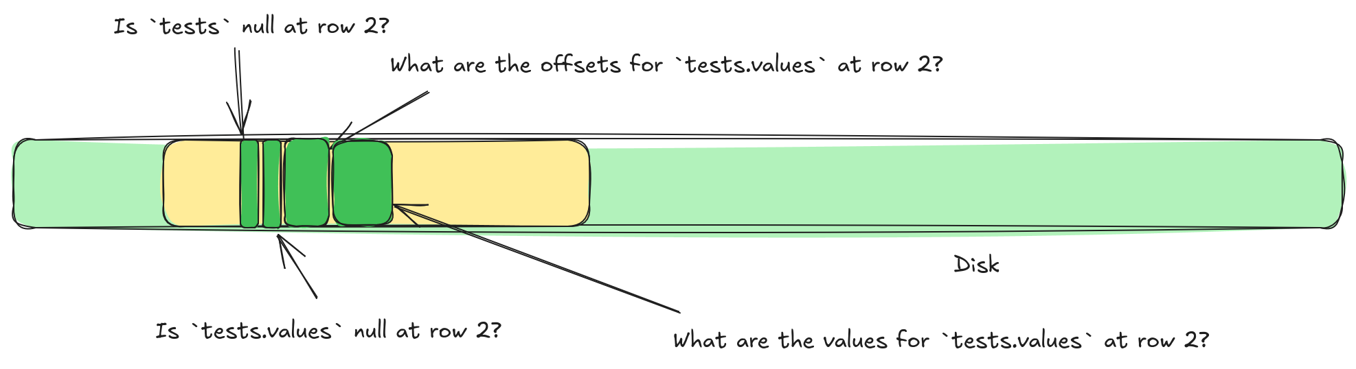
It turns out, we can sort of solve this problem, by reversing the shredding process after compression. Let's look at a concrete example. Let's imagine we want a single values list from our test file above. That list might be split into four different buffers, not even considering compression. We have the struct validity buffer, the list validity buffer, the list offsets buffer, and the list values buffer. This means we need to perform four different IOPS to grab this single list.

But what if we could stitch some of these buffers back together? For example, we could write a list offset, and then immediately write the validity. Or, if we switch to writing lengths we could write the list length, then the list validity, and then the list values. Can we even stitch the struct validity buffer in there somehow? What if we applied compression, could we stitch together different compression buffers?

It turns out the answer to all of these questions is "yes, sometimes". We call this stitching process "zipping" because it behaves very similarly to python's zip function. Here are the rules for zipping:

• If the compression is transparent we can zip compressed buffers back together.
• List offsets, list validity, and struct validity, can all be zipped together if we use something called repetition and definition levels (the next blog post in this series).
• If we zip together variable length items then we need something new called the "repetition index" (will be covered in a future blog post).

This is great news for random access. Sadly, it isn't free. All of this zipped data has to be unzipped when we read the data. The unzipping process can be costly. If the unzipping is too costly it can hurt our scan performance. All of this begs the question "when can we zip our data and when is the zipping too expensive?" This might sound a lot like the question "when can we use transparent encoding and when is it not worth it?" Once again, you'll need to stay tuned for the answer. We are getting closer, just a few more pieces to examine.

LanceDB is upgrading the modern data lake (postmodern data lake?). Support for multimodal data, combining search and analytics, embracing embedded in-process workflows and more. If this sort of stuff is interesting then check us out and come join the conversation.

Join us on Discord