Columnar File Readers in Depth: Compression Transparency

Conventional wisdom states that compression and random access do not go well together. However, there are many ways you can compress data, and some of them support random access better than others. Figuring out which compression we can use, and when, and why, has been an interesting challenge. As we've been working on 2.1 we've developed a few terms to categorize different compression approaches.

💡

This is part of a series of posts on building a columnar file reader. The series starts here and the most recent entry was here.

Setting the stage

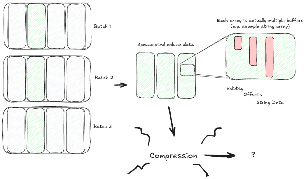
Compression in Lance happens on large chunks of data for a single array. As batches of data come in, we split those batches into individual columns, and each column queues up data independently. Once a column's queue is large enough, we trigger a flush for that column, and that initiates the compression process.

We don't have row groups, so we can accumulate columns individually, and flushing one column does not mean that we will be flushing other columns. This means, by the time we hit the compression stage, we typically have a large (8MB+ by default) block of column data that we need to compress.

Several batches of data on the left side, with multiple columns. The second column is highlighted. An arrow from this to the accumulated column data which is just the three highlighted columns on their own. An arrow from this to "compression" which is just some process. An arrow from this to ? which is the output of compression. An aside zooms in on a single column to point out that one column can have multiple buffers, for example, validity, offsets, and string data for a string array. — Each column accumulates arrays until it has enough data (8MB+) to justify creating a block.

Transparent vs. Opaque

The most impactful (for random access) distinction is determining whether an encoding is opaque or not. Opaque compression creates a block of data that must be fully decoded in order to access a single value. In contrast, transparent compression allows us to decompress a single value individually, without interacting with the other values in the block (to be clear, these are not industry standard terms, it's just what we use within Lance).

As a simple example, we can consider delta encoding. In delta encoding we only encode the difference between one value and the next. The deltas can often (but not always) be in a smaller distribution (and thus easier to compress) than the original values. Delta encoding is opaque. If I want the 6th value in a delta encoded array then I need to decode all of the values leading up to it (I suppose you could call this semi-opaque since we don't need to decode the values after it but that distinction is not useful for us).

Other opaque encodings include the "back referencing" family of encodings such as GZIP, LZ4, SNAPPY, and ZLIB. These encodings encode a value by encoding a "backwards reference" to a previous occurrence of that sequence. If you don't have the previous values you can't interpret this backward reference.

A graphical example showing the array [1, 2, 5, 6, 8, 9, 9, 11] compressed with delta encoding and bit packing into 3 bits per value. Starting value: 0x01000200050006000800090009000B00. Ending value 0b001001011001010001000010. The value 9 is highlighted in the array. It is 0x0900 in the plain array. It is spread across the range 0b001001011001010001 in the compressed array. — Delta encoding + bit packing gives great compression here. We go from 16 bytes to 3 bytes. However, our value gets "smeared" across a large portion of the data. We normally end up loading the entire block to decompress a single value.

To see an example of a transparent encoding we can look at bit packing. In bit packing we compress integer values that don't use up their whole range by throwing away unused bits. For example, if we have an INT32 array with the values [0, 10, 5, 17, 12, 3] then we don't need more than 5 bits per value. We can throw away the other 27 bits and save space.

This encoding is transparent (as long as we know the compressed width, more on that later) because, to get the 6th value, we know we simply need to read the bits bits[bit_width * 5..bit_width * 6]. I hope it is clear why this property might be useful for random access reads but we will be expanding on this more in a future post.

Example encoding the array [1, 2, 5, 6, 8, 9, 9, 11] with just bit packing. We go from 0x01000200050006000800090009000B00 to 0b00010010010101101000100110011011. The value 9 is highlighted. It is 0x0900 in the uncompressed buffer and 0b1001 in the compressed buffer. — Bit packing alone isn't as effective in this case, I end up with 4 bytes instead of 3, but it is transparent. If I want to load a single value I only need to read that one byte.

Can Variable Length Compression be Transparent?

Variable length layouts, for example, lists or strings, are not so straightforward. We typically need to do a bit of indirection to get the value, even when there is no compression. First, we look up the size of the value, then we look up the value itself. For example, if we have the string array ["compression", "is", "fun"] then we really (in Arrow world) have two buffers. The offsets array and the values array. Accessing a single value requires two read operations.

An example of the Arrow layout of the string array ["compression", "is", "fun"]. The offsets array ([0, 11, 13, 16]) is encoded as 0x00000B000D004000. The bytes array (compressionisfun) is encoded as 0x636F6D7072657373696F6E697366756E. The value "is" is highlighted. It needs the offsets 0x0B000D00 (11, 13) and the data bytes 0x6973 (is). — Variable length layouts require two buffer reads to access a single value

In our definition of transparent, we still consider this to be random access. Intuitively we can see that we still don't need the entire block to access a single value. As a result, we can have transparent variable length encodings. A very useful compression here is FSST. The details are complicated but FSST is basically partial dictionary encoding where the dictionary is a 256 byte symbol table. As long as you have that symbol table (this is metadata, discussed later) then you can decode any individual substring. This means that FSST encoding is, in fact, transparent.

The string array ["run", "spot run", "see spot", "run"] is encoded with a symbol table. The symbol table is 0x00=run, 0x01=spot, 0x02=see. The offsets are [0, 1, 3, 5, 6]. The bytes are 0x000100020100. — Using a symbol table we transparently create a compressed representation of a string array.

A more complete definition, which is what we've ended up with in our compression traits, is something like:

💡

For an encoding to be transparent then the result of the encoding must either be an empty layout, fixed width layout, or a variable width layout. The layout must have the same number of elements as the array. There may also optionally be one or more buffers of metadata. When decoding, if we have the metadata, we must be able to decode any element in the compressed layout individually.

We limit the layouts to empty, fixed width, and variable width because we know how to "schedule" those. We can convert an offset into one of those layouts into a range of bytes representing the data. We could potentially support additional layouts in the future.

🔜

Future Question: Just because we are given an 8MB chunk of data doesn't mean we have to compress the entire thing as one piece. We can break it up into smaller opaque chunks. Do we still get good compression with small chunks? Does this mean the opaque encoding can still be used with random access? How do we know which chunk to access? These are all valid questions and we will discuss these questions in a future post.

Mysterious "metadata"

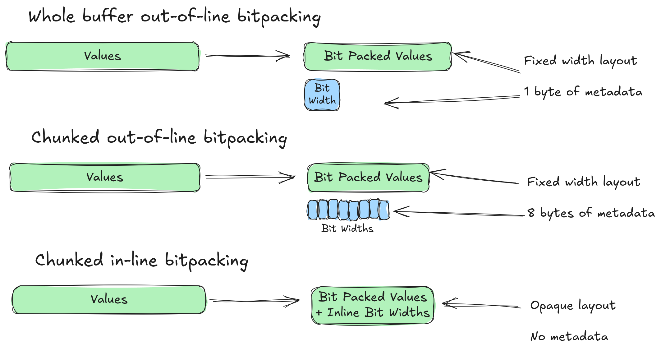
Our definition mentions "metadata", which isn't something we've talked about yet. However, it is critical when we look at random access. To understand, let's take another look at bit packing. I mentioned that we could decode the data transparently, as long as we knew the compressed bit width. How do we know this? We put it in the metadata. That means our naive bit packing algorithm has 1 byte of metadata.

Now lets look at a different way we could approach bit packing. To see why we might do this consider that we are encoding at least 8MB of integer data. What if we have just one large value in our array. That single outlier will blow our entire operation out of the water. There's lots of ways around this (e.g. replacing outliers with an unused value, moving outliers to metadata, etc.) but a simple one is to compress the data in chunks.

For simplicity let's pretend we compress it in eight 1MB chunks (chunks of 1024 values is far more common but this is a blog post and we don't want to think too hard). The chunk that has our outlier won't compress well but the remaining chunks will. However, each compressed chunk could have a different bit width. That means we now have 8 bytes of metadata instead 1 byte of metadata. Is this bad? The answer is "it depends" and we will address it in a future blog post.

A buffer of values contains an outlier. It is split into 8 chunks and bit packed. The compressed buffer of values is smaller and most of the chunks are tiny. The chunk containing the outlier is not much smaller. There is now also a metadata array of bit widths [5, 5, 5, 6, 6, 20, 6, 6]. The 20 represents the chunk with the outlier. — By chunking we can reduce the impact of an outlier. This is a general technique that applies to most compression algorithms. But now our bit width metadata is more extensive.

We can even eliminate metadata completely by making the compression opaque. All we need to do is inline the compressed bit width of a chunk into the compressed buffer of data itself. This is, in fact, the most common technique in use today, because random access has not typically been a concern. Putting all of this together we can see that a single technique (bit packing) can be implemented in three different ways, with varying properties (transparent vs. opaque, size of metadata).

A graphical representation of three styles of bit packing. In the first (whole buffer out-of-line bitpacking) a values array is turned into "bit packed values" (fixed width layout) and a tiny "bit width" (1 byte of metadata). The second (chunked out-of-line bitpacking) has a values buffer turn into a bit packed values buffer (fixed width layout) and a bigger bit widths buffer (8 bytes of metadata). The final (chunked in-line bitpacking) takes a values buffer and turns it into a single "bit packed values + inline bit width" buffer (opaque layout). There is no metadata in this approach. — Three different ways to compress with bitpacking showing tradeoffs between transparent/opaque and more/less metadata

Null Stripped vs. Null Filled

The next category considers how we handle nulls. We can either fill nulls or strip nulls. This is more or less independent of the compression we are using. When we compress something in a null stripped manner we remove the nulls before we compress the values. When we compress something in a null filled manner we insert garbage values in spots where nulls used to be. Those values can be anything and, in some cases, a compression algorithm might have a particular preference (e.g. when bit packing we probably don't want to put huge outlier values in null spots).

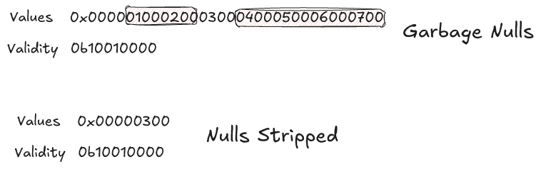
Two representations of an array. The first has garbage nulls. The values buffer is 0x00000100020003000400050006000700. The validity buffer is 0b10010000. The second has stripped nulls. The values buffer is 0x000003000. The validity buffer is the same. The garbage nulls in the first example are highlighted in red. — Two equally valid representations of the array [0, NULL, NULL, 3, NULL, NULL, NULL, NULL]

We can also see that stripping out nulls makes our compression opaque. In the above example we still have a fixed-width layout but we no longer have the right number of values. We have to walk through our validity bitmap in order to find the offset into our values buffer. This means we need the entire validity bitmap before we can decode any single value.

❓

Challenge Exercise: What if we had a mostly-null array and we decided to speed things up by declaring the validity buffer to be metadata? After all, this could just a compressed bitmap, it's probably not too large. Would this be transparent? Does it meet our definition above? Is this good or bad? How large is too large?

👾

This garbage data is rarely very large. Fixed size types tend to be quite small. Variable-width types don't need "garbage bytes". They only need a garbage offset (and actually, it's not really garbage, it must equal the previous offset).

One curious exception to this rule is vector embeddings as they are both fixed-size and quite large (typically 3-6KB)

Another (perhaps obvious) exception is mostly-null arrays.

Putting it in Action: Parquet & Arrow

In Parquet our block equivalent is the column chunk. Parquet divides the column chunk into pages (similar to the chunked bit packing example above) and it assumes all compression is opaque. As a result, Parquet is able to strip nulls before compression. However, when we perform random access into a Parquet column we must always read an entire page.

In Arrow's memory format, there isn't really much compression (the IPC format supports some opaque buffer compression). However, it is important in Arrow that random access be reasonably fast. All of the layouts are transparent. Arrow does not remove nulls and it must fill nulls with garbage values. However, with most arrays, we can access a single value in O(1) read operations. Bonus challenge: At the moment there is exactly one exception to these rules. Do you know what it is?

Conclusion: Which is best?

I work on Lance, a file format that is aiming to achieve fast full scan and random access performance. You probably think my answer will be that we need to switch everything to use transparent compression and then are expecting some statement about minimizing metadata. Unfortunately, it's not quite that simple. Sometimes we find ourselves in situations where we can use opaque metadata. Sometimes more metadata is a good thing. We're going to need to explore a few more concepts before we can really evaluate things. It's probably bad form to end a blog without actually answering anything but 🤷

See you next time.

LanceDB is upgrading the modern data lake (postmodern data lake?). Support for multimodal data, combining search and analytics, embracing embedded in-process workflows and more. If this sort of stuff is interesting then check us out and come join the conversation.

Join us on Discord