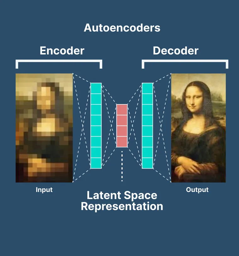
Autoencoders encode an input into a latent space and decode the latent representation into an output. The output is often referred to as the reconstruction, as the primary goal is to reconstruct the input from the latent code.
Autoencoders are a very popular for data compression due to their ability to efficiently capture and represent the essential features of the input data in a compact form.
One problem that autoencoders face is the lack of variation. This means that while they can effectively compress and reconstruct data, they struggle to generate new, diverse samples that resemble the original data. The latent space learned by traditional autoencoders can be sparse and disjointed, leading to poor generalization and limited ability to produce meaningful variations of the input data.
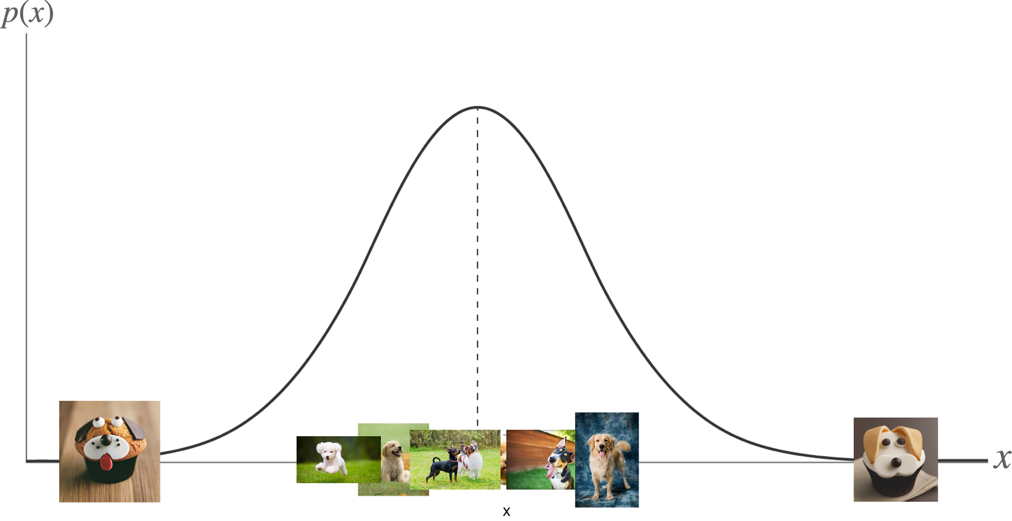
What do we mean by variation?
In the context of generative models, variation refers to the ability to produce a diverse range of outputs from a given latent space. For instance, in image generation, variation means creating different but plausible images that share common characteristics with the training data.
Traditional autoencoders, while good at reconstruction, do not inherently encourage this diversity. They tend to map inputs to specific points in the latent space, which can limit the model's ability to explore and generate new samples.
Introducing Variational Autoencoders (VAEs) as a Solution: Variational Autoencoders (VAEs) address this limitation by introducing a probabilistic approach to the encoding process. Instead of mapping inputs to fixed points in the latent space, VAEs map inputs to a distribution over the latent space. This allows for a smoother and more continuous representation of the data, fostering better generalization and enabling the generation of diverse outputs.
Here's a high-level overview of how VAEs work:
- Encoder: Maps the input data to a mean and variance that define a Gaussian distribution in the latent space.
- Sampling: Samples a point from this Gaussian distribution.
- Decoder: Uses the sampled point to reconstruct the input data, ensuring that the output is a plausible variation of the input.
In the next sections of this blog post, we talk about the technical details of setting up and training a VAE. We will also explore how the Lance data format can be leveraged to optimize data handling, ensuring efficient and scalable workflows.
By integrating VAEs with Lance, you can unlock new possibilities in data compression, generation, and management, pushing the boundaries of what is achievable with machine learning.
Setup and Imports
We begin with setting up our imports for the experiment.
$ pip install -U -q pylanceimport torch
import torch.nn as nn
import torch.optim as optim
from torch.utils import data
import torchvision.transforms as transforms
from torch.utils.data import DataLoader
from torchvision.datasets import ImageFolder
import io
from PIL import Image
from tqdm import tqdm
from matplotlib import pyplot as plt
import requests
import tarfile
import os
import time
import pyarrow as pa
import lanceConfiguration
We will now configure our experiment. Please feel free to change the configuration and run the experiment on your own to see what changes! This is a great exercise to indulge in.
vae_config = {
    "BATCH_SIZE": 4096,
    "IN_RESOLUTION": 32,
    "IN_CHANNELS": 3,
    "NUM_EPOCHS": 100,
    "LEARNING_RATE": 1e-4,
    "HIDDEN_DIMS": [64, 128, 256, 512],
    "LATENT_DIM_SIZE": 64,
}
Dataset
This section of the blog post is taken from Lance Deep Learning Recepies.
Here we will download the CINC-10 dataset and convert it into a Lance dataset. After we have that, we will use our PyTorch dataloader to load the dataset into our training pipeline.
# Define the URL for the dataset file
data_url = "https://datashare.ed.ac.uk/bitstream/handle/10283/3192/CINIC-10.tar.gz"

# Create the data directory if it doesn't exist
data_dir = "cinic-10-data"
if not os.path.exists(data_dir):
    os.makedirs(data_dir)

# Download the dataset file
print("Downloading CINIC-10 dataset...")
data_file = os.path.join(data_dir, "CINIC-10.tar.gz")

response = requests.get(data_url, stream=True)
total_size = int(response.headers.get('content-length', 0))
block_size = 1024

start_time = time.time()
progress_bar = tqdm(total=total_size, unit='iB', unit_scale=True)

with open(data_file, 'wb') as f:
    for chunk in response.iter_content(chunk_size=block_size):
        if chunk:
            f.write(chunk)
            progress_bar.update(len(chunk))

end_time = time.time()
download_time = end_time - start_time
progress_bar.close()

print(f"\nDownload time: {download_time:.2f} seconds")

# Extract the dataset files
print("Extracting dataset files...")
with tarfile.open(data_file, 'r:gz') as tar:
    tar.extractall(path=data_dir)

print("Dataset downloaded and extracted successfully!")
def process_images(images_folder, split, schema):
# Iterate over the categories within each data type
label_folder = os.path.join(images_folder, split)
for label in os.listdir(label_folder):
label_folder = os.path.join(images_folder, split, label)
# Iterate over the images within each label
for filename in tqdm(os.listdir(label_folder), desc=f"Processing {split} - {label}"):
# Construct the full path to the image
image_path = os.path.join(label_folder, filename)
# Read and convert the image to a binary format
with open(image_path, 'rb') as f:
binary_data = f.read()
image_array = pa.array([binary_data], type=pa.binary())
filename_array = pa.array([filename], type=pa.string())
label_array = pa.array([label], type=pa.string())
split_array = pa.array([split], type=pa.string())
# Yield RecordBatch for each image
yield pa.RecordBatch.from_arrays(
[image_array, filename_array, label_array, split_array],
schema=schema
)
# Function to write PyArrow Table to Lance dataset
def write_to_lance(images_folder, dataset_name, schema):
for split in ['test', 'train', 'valid']:
lance_file_path = os.path.join(images_folder, f"{dataset_name}_{split}.lance")
reader = pa.RecordBatchReader.from_batches(schema, process_images(images_folder, split, schema))
lance.write_dataset(
reader,
lance_file_path,
schema,
)
dataset_path = "cinic-10-data"
dataset_name = os.path.basename(dataset_path)
start = time.time()
schema = pa.schema([
pa.field("image", pa.binary()),
pa.field("filename", pa.string()),
pa.field("label", pa.string()),
pa.field("split", pa.string())
])
start = time.time()
write_to_lance(dataset_path, dataset_name, schema)
end = time.time()
print(f"Time(sec): {end - start:.2f}")Build a small utility to visualize our data and the generated images from the model.
def draw_image_grid(samples):
    images = samples[:4]
    images = (images * 0.5) + 0.5  # Unnormalize the images to [0, 1] range
    grid_img = torchvision.utils.make_grid(images, nrow=2)
    plt.figure(figsize=(5, 5))
    plt.imshow(grid_img.permute(1, 2, 0))  # Convert from (C, H, W) to (H, W, C)
    plt.axis('off')
    plt.show()
Let us now build the Data Generator
class CustomImageDataset(data.Dataset):
    def __init__(self, classes, lance_dataset, transform=None):
        self.classes = classes
        self.ds = lance.dataset(lance_dataset)
        self.transform = transform

    def __len__(self):
        return self.ds.count_rows()

    def __getitem__(self, idx):
        raw_data = self.ds.take([idx], columns=['image', 'label']).to_pydict()
        img_data, label = raw_data['image'][0], raw_data['label'][0]

        img = Image.open(io.BytesIO(img_data))

        # Convert grayscale images to RGB
        if img.mode != 'RGB':
            img = img.convert('RGB')

        if self.transform:
            img = self.transform(img)

        label = self.classes.index(label)
        return img, label
To instantiate a data loader we use the following code.
train_transform = transforms.Compose(
    [
        transforms.ToTensor(),
        transforms.Normalize((0.5, 0.5, 0.5), (0.5, 0.5, 0.5)), # -1 to 1
    ]
)
classes = ('airplane', 'automobile', 'bird', 'cat', 'deer', 'dog', 'frog', 'horse', 'ship', 'truck')

lance_train_dataset = CustomImageDataset(
    classes,
    "cinic-10-data/cinic-10-data_train.lance/",
    transform=train_transform
)

lance_train_loader = torch.utils.data.DataLoader(
    lance_train_dataset,
    batch_size=vae_config["BATCH_SIZE"],
    shuffle=True
)
Time to visualize our dataset.
images, _ = next(iter(lance_train_loader))
draw_image_grid(images)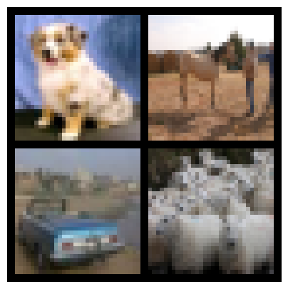
Building the model
A Variational Autoencoder (VAE) is very similar to a standard autoencoder in its structure and basic functionality. Both models consist of an encoder and a decoder. The encoder compresses the input into a latent representation, and the decoder reconstructs the input from this latent code. However, VAEs introduce several critical modifications that address some of the limitations of standard autoencoders, particularly regarding the generation of diverse and meaningful outputs.
Key Components of the Variational Autoencoder
- Encoder: The encoder in a VAE consists of several convolutional layers (in the case of images) that transform the input data into a lower-dimensional latent space. The encoder outputs the mean and variance parameters of the latent distribution, rather than a fixed latent code.
- Reparameterization: The reparameterization trick allows the model to sample from the latent distribution in a differentiable manner. This step involves sampling a latent code from the Gaussian distribution defined by the mean and variance parameters output by the encoder.
- Decoder: The decoder takes the sampled latent code and reconstructs the input data. It consists of several deconvolutional layers that gradually upsample the latent code back to the original input dimensions.
- Loss Function: The VAE loss function comprises the reconstruction loss and the KL divergence loss. The reconstruction loss ensures that the output is a faithful reconstruction of the input, while the KL divergence loss regularizes the latent space.
Here's a high-level summary of how a VAE operates:
- Encoding: The input is passed through the encoder, which outputs the mean and variance of the latent distribution.
- Sampling: A latent code is sampled from this distribution using the reparameterization trick.
- Decoding: The sampled latent code is passed through the decoder to reconstruct the input.
- Loss Calculation: The loss function, combining reconstruction loss and KL divergence loss, is used to optimize the model.
By incorporating these probabilistic elements and regularization techniques, VAEs overcome some of the limitations of traditional autoencoders, particularly in terms of generating diverse and meaningful outputs. In the next sections, we will explore the technical implementation of a VAE, leveraging the Lance data format to optimize data handling and improve the efficiency of our workflows.
# VAE Model
class VAE(nn.Module):
    def __init__(self):
        super(VAE, self).__init__()

        # Encoder
        self.encoder = nn.Sequential(
            nn.Conv2d(vae_config["IN_CHANNELS"], 32, kernel_size=4, stride=2, padding=1),
            nn.ReLU(),
            nn.Conv2d(32, 64, kernel_size=4, stride=2, padding=1),
            nn.ReLU(),
            nn.Conv2d(64, 128, kernel_size=4, stride=2, padding=1),
            nn.ReLU(),
            nn.Flatten()
        )

        self.fc_mu = nn.Linear(128*4*4, vae_config["LATENT_DIM_SIZE"])
        self.fc_logvar = nn.Linear(128*4*4, vae_config["LATENT_DIM_SIZE"])

        # Decoder
        self.decoder_input = nn.Linear(vae_config["LATENT_DIM_SIZE"], 128*4*4)

        self.decoder = nn.Sequential(
            nn.ConvTranspose2d(128, 64, kernel_size=4, stride=2, padding=1),
            nn.ReLU(),
            nn.ConvTranspose2d(64, 32, kernel_size=4, stride=2, padding=1),
            nn.ReLU(),
            nn.ConvTranspose2d(32, vae_config["IN_CHANNELS"], kernel_size=4, stride=2, padding=1),
            nn.Tanh()  # Output values in range [-1, 1]
        )

    def reparameterize(self, mu, logvar):
        std = torch.exp(0.5 * logvar)
        eps = torch.randn_like(std)
        return mu + eps * std

    def forward(self, x):
        x = self.encoder(x)
        mu = self.fc_mu(x)
        logvar = self.fc_logvar(x)
        z = self.reparameterize(mu, logvar)
        z = self.decoder_input(z)
        z = z.view(-1, 128, 4, 4)
        return self.decoder(z), mu, logvar

    def sample(self, num_samples):
        z = torch.randn(num_samples, vae_config["LATENT_DIM_SIZE"]).to(device)
        return self.decoder(self.decoder_input(z).view(-1, 128, 4, 4))
Time to TRAIN!
device = "cuda"

# Loss Function
def vae_loss(recon_x, x, mu, logvar):
    recon_loss = nn.functional.mse_loss(recon_x, x, reduction='sum')
    kl_loss = -0.5 * torch.sum(1 + logvar - mu.pow(2) - logvar.exp())
    return recon_loss + kl_loss

# Initialize model, optimizer
model = VAE().to(device)
optimizer = optim.Adam(model.parameters(), lr=vae_config["LEARNING_RATE"])
for epoch in range(vae_config["NUM_EPOCHS"]):
model.train()
train_loss = 0
# Use tqdm for the progress bar
pbar = tqdm(enumerate(lance_train_loader), total=len(lance_train_loader), desc=f'Epoch {epoch+1}/{vae_config["NUM_EPOCHS"]}')
for batch_idx, (data, _) in pbar:
data = data.to(device)
optimizer.zero_grad()
recon_batch, mu, logvar = model(data)
loss = vae_loss(recon_batch, data, mu, logvar)
loss.backward()
train_loss += loss.item()
optimizer.step()
# Update tqdm description with current loss
pbar.set_postfix({'Loss': loss.item()})
avg_loss = train_loss / len(lance_train_loader.dataset)
print(f'Epoch [{epoch + 1}/{vae_config["NUM_EPOCHS"]}] Average Loss: {avg_loss:.4f}')
# show and display a sample of the reconstructed images
if epoch % 10 == 0:
with torch.no_grad():
sampled_images = model.sample(num_samples=4)
draw_image_grid(recon_batch.cpu())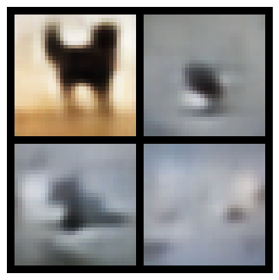
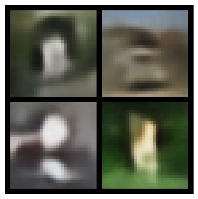
The images generated from the training pipeline are not bad! You have to note that the generations follow the centred theme as that of the dataset. We also see the green grass and blue skies in some images.
Train it longer to see how the model converges!
Let's see the reconstruction
images, _ = next(iter(lance_train_loader))
draw_image_grid(images)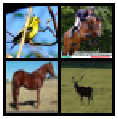
with torch.no_grad():
    recon_images, _, _ = model(images.to(device))
draw_image_grid(recon_images.cpu())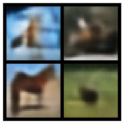
Conclusion
In this tutorial, we understood what Variational Autoencoder are, and how to train them. We have also use the powerful lance data fomat for our training pipeline which make the training easier and more efficient.